Supercharged high-resolution ocean simulation with JAX

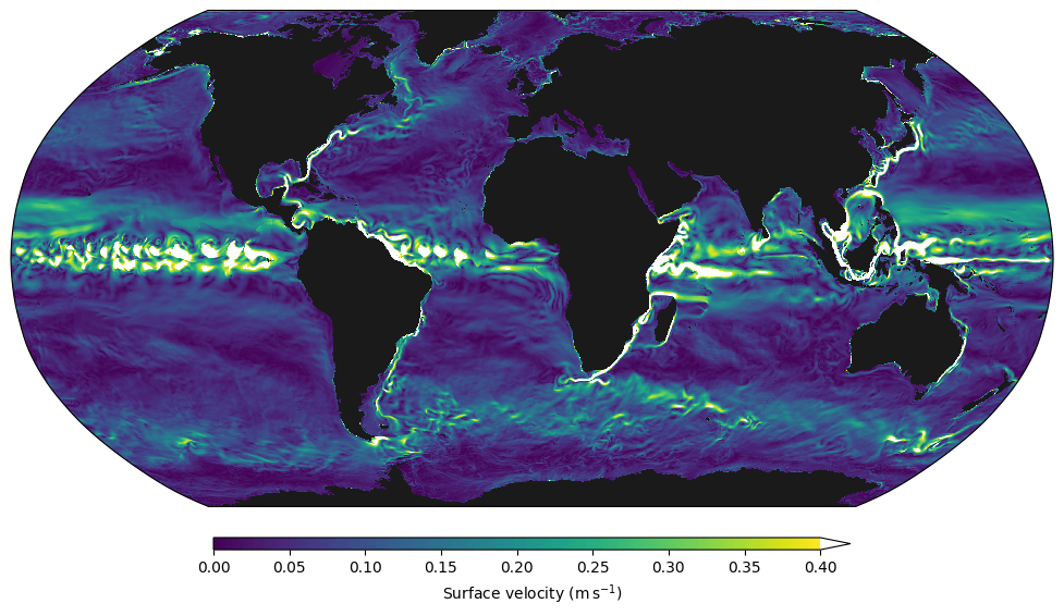
Our Python ocean model Veros (which I maintain) now fully supports JAX as its computational backend. As a result, Veros has much better performance than before on both CPU and GPU, while all model code is still written in Python. In fact, we can now do high-resolution ocean simulations on a handful of GPUs, with the performance of entire CPU clusters!

So, what does this mean, and how did we pull this off? In this blog post I will give you an introduction to high-performance ocean modelling, show you how JAX fits into the picture, and show some benchmarks to prove to you that Python code can be competitive with hand-written Fortran (while also having great GPU performance).

If you want to know all the details, you should make sure to also check out our article “Fast, cheap, & turbulent — Global ocean modelling with GPU acceleration in Python” that was published in the Journal of Advances in Earth System Modelling (JAMES) today.

Ocean modelling in a nutshell¶

Ocean models simulate how the oceans react to external forcings, like irradiation from the sun, wind patterns, or freshwater influx from rivers and glaciers. As such, they are a major component of every climate model (other parts being for example atmosphere, ice, and land models), and help us understand the complex processes taking place in the real oceans.

In the following sections I will show you how oceans can be modelled mathematically, and how we can solve these equations with computers, before we dive deeper into using JAX for high-performance computing.

The primitive equations¶

The starting point for almost all fluid dynamics are the Navier-Stokes and continuity equations, which are derived from momentum and mass conservation within the fluid. In their most general form these equations are too unwieldy for ocean modelling, but after a few reasonable approximations (like assuming a constant background density and small vertical velocities), we arrive at the so-called primitive equations.

I won’t go into too much detail here, but I think it is still nice to show the equations in full so you can get an idea of the complexity of the problem we are trying to solve. They can be written like this:

This is a set of 7 coupled, nonlinear partial differential equations. The primitive equations describe the evolution of velocity \(\vec{v} = (u, v, w)\) (\(\vec{v_h} = (u, v)\)), pressure \(p\), density \(\rho\), temperature \(\theta\), and salinity \(S\) in time \(t\) and space \((x, y, z)\). \(f, \rho_0\), and \(g\) are constants; and \(\vec{\mathcal{F}}\), \(\mathcal{Q}_\theta\), and \(\mathcal{Q}_S\) represent dissipation and forcings (which are usually quite complex terms, too).

So how can we even solve complex equations like these on a computer? One of the simplest ways is to discretize them using a finite difference method.

Discretization¶

The basic idea is to define all quantities (like pressure and velocity) at fixed locations on a computational grid. This implies that we are now dealing with discrete quantities \((y_0, y_1, \ldots, y_N)\) instead of their true continuous versions \(y(x)\). If you are familiar with calculus, you probably know that a derivative can be written as a difference between neighboring grid cells, divided by a small step size:

This converges to the “true” value in the limit of smaller and smaller \(\Delta x\). Writing gradients like this is the central idea of finite difference discretizations, and although there are many different ways to write these discrete gradients — with different numerical accuracies and stability properties — the principle is always the same.

For time derivatives, we typically use a multi-step method:

This requires us to store the solution at different time steps, but is otherwise not more difficult than a simple forward difference.

By replacing all gradients in the primitive equations through their discrete counterparts, we arrive at a set of discrete equations that can be stepped forward in time. To solve them on a computer, all we need to do is to define our physical variables as arrays (where array indices correspond to grid locations), and perform the right finite difference operations. For example, in vectorized Python code, we can write a gradient operation like the one above through index shifts:

# discrete version of ∂y/∂x
#
#             y_{i+1}   y_{i}
#                |        |
dy_dx[1:-1] = (y[2:] - y[1:-1]) / dx

For this to work, we need to pad all arrays by 1 extra element along each dimension (so the original data is y[1:-1]). Then, we can compute finite differences by shifting slices. The extra elements y[0] and y[-1] are called “ghost cells” or “overlap”.

Parallelization¶

Solving the primitive equations is very computationally expensive. Our model domain is typically the whole globe, and the non-linear nature of the primitive equations impose tight constraints on the largest time steps we can take. To make things worse, the ocean has a long memory of hundreds of years, so we need to run very long simulations until they reach a steady state — it’s not uncommon that a setup runs for more than 1 million time steps.

Because of this, even relatively low-resolution models like 3×3° (with about 600,000 grid elements) should be run on more than one process, unless you are willing to wait on results for months. High-resolution setups typically run on thousands of processes (CPU cores) across dozens of computational nodes.

The basic idea to execute the model in parallel is a simple domain decomposition. Every process takes ownership of a chunk of the total domain, and iterates it forward in time. Of course, neighboring processes need to exchange information from time to time, e.g. by sending messages through MPI (Message Passing Interface). Luckily, we can re-use our overlap cells for this! So by filling the ghost cells of each chunk with the current solution from the process neighbor we can ensure that the final solution is identical to that of the sequential model. This process is also called halo exchange.

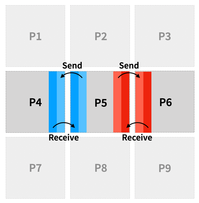
How often communications need to happen depends on how far each index is shifted, and the size of the overlap region. An overlap of 2 on each edge gives us enough leeway to execute 2 forward operations on the same array before having to communicate.

Now we are ready solve the primitive equations on an arbitrary number of processes with vectorized array operations. JAX is an excellent fit for this task, as we will see in the next section.

JAX for high-performance computing¶

Even though most people use JAX for machine learning, it is actually a great choice for high-performance computing. Through its just-in-time (JIT) compiler, JAX has good all-round performance on CPU and GPU, and the API is close enough to NumPy to make it easy to port existing code.

To demonstrate how this works in practice, I will show you how to implement the time stepping for a simple partial differential equation in JAX. Here is the equation, and the resulting JAX code:

# compile function with jit for speed
@jax.jit
def update_h(h, dh, fe, fn):
    """Step h forward in time."""

    # compute right hand side
    dh_new = dh.at[1:-1, 1:-1].set(
        -(fe[1:-1, 1:-1] - fe[1:-1, :-2]) / dx
        - (fn[1:-1, 1:-1] - fn[:-2, 1:-1]) / dy
    )

    # step in time via multistep integration
    h = h.at[1:-1, 1:-1].add(
        dt * (1.5 * dh_new[1:-1, 1:-1] - 0.5 * dh[1:-1, 1:-1])
    )

    # enforce cyclic boundaries and handle inter-process communication
    h = enforce_boundaries(h)
    return h

Applying this function to a model state with variables {h, dh, fe, fn} yields a new state, with h stepped forward in time by dt. And because we can write finite difference operations in a fully vectorized way with JAX (via index shifts), the implementation ends up clean and fast.

The only big obstacle left to figure out is communication between processes — i.e., what happens inside enforce_boundaries. In functions decorated with @jax.jit, arrays can only be manipulated through transformations that are known to the underlying compiler, XLA. This means that we would have to break control flow at every communication operation to leave JIT, perform the operation, and then re-enter a JIT block. This is ugly: it complicates the code structure, and we are leaving performance on the table by applying JIT to smaller blocks at a time.

To solve this problem I co-developed mpi4jax, which registers MPI operations with XLA, so we can use them within JIT blocks. Here is a simplified implementation of enforce_boundaries, where we use mpi4jax.sendrecv to exchange information:

@jax.jit
def enforce_boundaries(arr, grid):
    """Exchange overlap between processes."""
    token = None
    send_order = ("west", "east")
    recv_order = ("east", "west")

    # loop over neighbors
    for send_dir, recv_dir in zip(send_order, recv_order):
        # determine neighboring processes
        send_proc = proc_neighbors[send_dir]
        recv_proc = proc_neighbors[recv_dir]

        # determine data to send
        send_idx = overlap_slices_send[send_dir]
        send_arr = arr[send_idx]

        # determine where to place received data
        recv_idx = overlap_slices_recv[recv_dir]
        recv_arr = jnp.empty_like(arr[recv_idx])

        # execute send-receive operation through mpi4jax
        recv_arr, token = mpi4jax.sendrecv(
            send_arr,
            recv_arr,
            source=recv_proc,
            dest=send_proc,
            comm=mpi_comm,
            token=token,
      )

        # update array with received data
        arr = arr.at[recv_idx].set(recv_arr)

      return arr

(for a full, working example see the mpi4jax repository)

With this in place, we can do fully distributed simulations on CPU and GPU, with just a few lines of Python code.

Veros + JAX in action¶

Because the whole model is written in Python, getting started with Veros is pretty easy. For example, if you already have a working Python installation and current CUDA drivers, the following screencast shows you all you need to do to:

1. Install Veros and all dependencies
2. Run a global 1x1° setup on GPU

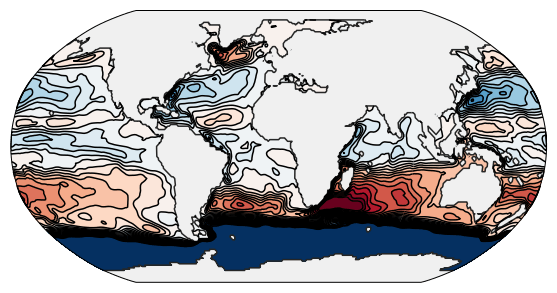
Leaving this setup running on a high-end GPU for about 24 hours finally leads to output like this, which shows us all the major ocean circulations:

Similarly, we can run Veros on multiple CPU cores (in this case 4) like this:

$ mpirun -n 4 veros run global_1deg -b jax -n 2 2

(after installing MPI, mpi4py, and mpi4jax)

Turns out it’s pretty fast¶

Now we can finally run some benchmarks of the new JAX backend. Because the dynamical core of Veros is a one-to-one translation of a Fortran model to Python, we can also do a direct comparison between JAX and the original Fortran code.

First up, we compare the performance on a single computer with 24 CPU cores and a Tesla P100 GPU. This benchmark shows you how the computational efficiency depends on the number of grid elements:

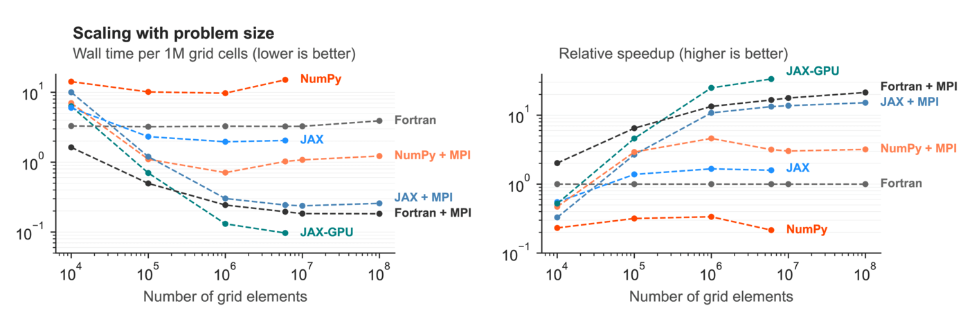
We can see that single-process NumPy is 3-4x slower than single-process Fortran, while JAX is a bit faster (mostly because JAX has some thread parallelism under the hood). On all 24 CPU cores, JAX is marginally slower than Fortran, while JAX on GPU outperforms everything.

But this is only what we get on a single computational node. Realistic ocean models need to run much faster than that, so we have to study how Veros scales to multiple nodes in a compute cluster. For CPU, we measured this:

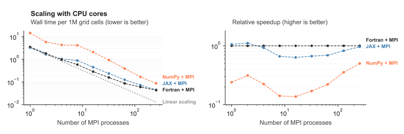
Again, JAX is only slightly slower than Fortran or breaks even, with NumPy far behind. This means that we are able to match the performance of Fortran, a highly optimized language made for high-performance computing, with our pure Python model + the JAX compiler, without any of the baggage that comes with Fortran models.

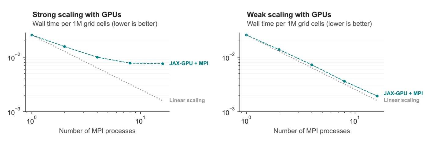
But the real star is this benchmark, where we see how Veros / JAX scales to multiple GPUs:

These results are a bit difficult to unpack, but the gist is this: If we can decompose the computational domain in such a way that every GPU is fully utilized, scaling to more devices is almost perfect. This is what allowed us to run a very high resolution simulation (global 0.1°) on a single Google Cloud instance with 16 GPUs — which people typically run on at least 2000 Fortran processes. You could already see the result at the start of this article, but here it is again:

Differentiable physics¶

Now that we have a fast ocean model in Python, what’s next? Most of all, I hope that people will simply find Veros enjoyable to work with, and use it to understand our earth and climate.

But there is one more new, interesting direction, namely the integration of machine learning models into the physical simulation. This is possible because JAX offers more than just a JIT compiler: JAX functions are also differentiable, which opens up a whole new of possibilities (Veros is not fully differentiable yet, but could be with some more effort).

In particular, there is an emerging field of physics-based deep learning that integrates machine learning with physical modelling. In case of a differentiable physical model, these “hybrid” systems can be trained end-to-end, which tends to make training much more efficient. There are already differentiable models for fluid dynamics in JAX (namely PhiFlow and jax-cfd), but — as far as I know — Veros is the first that supports realistic ocean setups.

Finally, I hope that I managed to share some of my excitement about working on modern physical models! If so, you are welcome to contribute.