(Niels Bohr Institute, Copenhagen, Denmark)
This post is the display material for the vEGU 2021 abstract “Higher-level geophysical modelling” in session AS1.1 (Recent Developments in Numerical Earth System Modelling).
Therefore, it is a bit more technical than my usual blog posts, and assumes that you are somewhat familiar within the field of numerical modelling.
A paradigm shift
The year is 2021, but numerical modelling and high-performance computing are still bastions of low-level programming languages. Most (finite difference) models are written in Fortran or C, which have been around since the early days of computing.
This is not surprising on the very largest compute scales like the CMIP climate model ensembles, which run on the world’s largest supercomputers. In this case, even small performance drops could end up consuming funding for several human positions. But this is an extreme example, and typically, human time tends to be more valuable than computer time. (Just think of your poor PhD students trying to compile the model code or get their setup to work.)
On top of this, the efficiency of GPUs has increased dramatically in tandem with the recent machine learning boom. This has also lead to more heterogeneous compute architectures than ever. For example, Finland’s LUMI supercomputer will consist of 550 PFLOP/s worth of GPUs (on top of about 200,000 CPU cores).
We think that these two developments call for a new, flexible generation of geophysical models:
- Flexible to run. The same code needs to be able to run on CPU and GPU hardware stacks.
- Flexible to use. Simple to install and get started.
- Flexible to modify. Readable code with helpful abstractions. Easy to re-build.
- Flexible to integrate. Simple to interface with external libraries for plotting, post-processing, machine learning, other models, …
We call these flexible models “high-level”, and to meet these design goals, at least a part of them needs to be implemented in a high-level programming language.
The taxonomy of high-level modelling
Essentially, high-level modelling comes in 3 different flavors. Each of these is a good way forward, and definitely a step up from the status quo.
-
Type I: High-level frontend, low-level backend
A typical example is climt, an atmospheric model that wraps modular computational kernels written in Fortran with a Python user interface, or PyOM2, an ocean model with a similar structure.
Those models have great CPU performance out of the box, and are straightforward to implement.
Our biggest concern with models of this type is the lack of GPU support. Developers need to maintain a seperate backend implementation, for example in CUDA, to run on GPU. Developing and maintaining 2 implementations of the same code is more than many academic projects can handle.
-
Type II: High-level model in a niche programming language
This is the approach pursued by the Climate Modelling Alliance‘s Oceananigans.jl model, implemented in Julia.
Julia in particular has excellent performance, first-class GPU support, and a growing scientific library ecosystem. Therefore, it has tremendous potential to become the dominant language for scientific computing.
On the other hand, Julia’s focus on scientific applications is both blessing and curse. In this day and age, a lot of the progress in computing is driven by applications outside academia (mostly through machine learning). Sticking to a programming language that is not (yet) widely established means that such synergies can’t be exploited.
-
Type III: High-level model in a widely used programming language
Currently, Python is the only programming language that fits this category. Python is being used extensively both inside and outside academia, and probably has the largest scientific library ecosystem of any programming language.
The only example we know for this type is our Python ocean model Veros. (We’re sure there’s more - if you know or maintain a high-performance model in Python, please reach out.)
Although we have the highest respect for Type I and II projects, we argue that Type III is the most valuable type of model, because it is easier to use / modify (more people are already familiar with the language and ecosystem) and integrate (larger library support) than the other types.
If you need some evidence for that last statement, just look how easy it is to install and use Veros from a clean Linux environment:
Installing and running Veros, starting from a fresh environment. Screencast in real time. Unfortunately, this type is also the hardest to get right. The main problem is finding the right trade-off between readability, performance, and abstraction.
For the remainder of this blog post, we will discuss what it takes to build high-performance models in Python, and where we should go as a community to make this as painless as possible.
Let’s talk about performance
Model performance is the elephant in the room whenever we discuss high-performance computing in Python.
As we argue in the introduction, human time is often more valuable than computer time, so we don’t think that it should be prioritized at all cost. However, model performance is a part of the user experience. A long feedback loop between designing an experiment and examining its results is catastrophic to overall productivity.
So, we have to care about performance to some degree. Luckily, this is largely a solved problem. It is already possible to match native Fortran performance in Python (within ±10%).
Pure Python / NumPy is of course nowhere close to Fortran — in our experience, a model written in NumPy is about 5x slower than its Fortran equivalent. But fortunately, there is a rich library ecosystem to accelerate Python code. Most of these libraries are geared towards machine learning, but nothing prevents us from using them for scientific computing instead. (Remember when we mentioned synergy as a major asset of Type III models?)
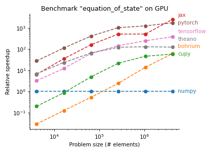
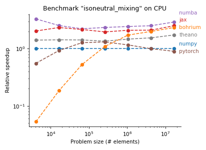
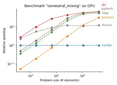
The following plots are from pyhpc-benchmarks, a repository we created to compare the performance of various Python frameworks on subroutines of our ocean model Veros:
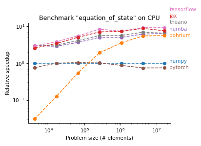
There are two Python frameworks that show particularly strong performance, Numba and JAX. To give you an idea how this works, here is the same code snippet in Fortran, NumPy, Numba, and JAX:
Fortran
tke_surf_corr = 0.0
do j=js_pe,je_pe
  do i=is_pe,ie_pe
    if (tke(i,j,nz,taup1) < 0.0 ) then
      tke_surf_corr(i,j) = -tke(i,j,nz,taup1)*(0.5*dzw(ke)) /dt_tke
      tke(i,j,nz,taup1) = 0.0
    endif
  enddo
enddo
NumPy
mask = tke[2:-2, 2:-2, -1, taup1] < 0.0
tke_surf_corr = np.zeros_like(maskU[..., -1])
tke_surf_corr[2:-2, 2:-2] = np.where(
    mask,
    -tke[2:-2, 2:-2, -1, taup1] * 0.5 * dzw[-1] / dt_tke,
    0.
)
Numba
tke_surf_corr = np.zeros((nx, ny))
for i in range(2, nx-2):
    for j in range(2, ny-2):
        if tke[i, j, -1, taup1] >= 0.:
            continue
        tke_surf_corr[i, j] = -tke[i, j, -1, taup1] * (0.5 * dzw[-1]) / dt_tke
        tke[i, j, -1, taup1] = 0.
JAX
mask = tke[2:-2, 2:-2, -1, taup1] < 0.0
tke_surf_corr = jnp.zeros_like(maskU[..., -1])
tke_surf_corr = tke_surf_corr.at[2:-2, 2:-2].set(
    jnp.where(
        mask,
        -tke[2:-2, 2:-2, -1, taup1] * 0.5 * dzw[-1] / dt_tke,
        0.
    )
)
See how the Numba implementation is basically translated Fortran, including the explicit loops? Numba’s JIT compiler is very efficient at transforming explicit loops like this one, essentially giving us the same performance as the Fortran code after compilation.
Unfortunately, there is no way to use the same Numba implementation for both CPU and GPU, as efficient GPU code generation typically requires a vectorized approach instead of explicit loops.
JAX on the other hand reads very similarly to NumPy, but its JIT compiler generates code that is competitive with Numba / Fortran on CPU and has great performance on GPU (with speedups of 40x — 3000x over NumPy). The only major restrictions are that JAX arrays are immutable and all JAX functions have to be pure (i.e., have no side effects).
We have therefore decided on JAX as the new computational backend for Veros. First benchmarks of the full model show that, with JAX, high-resolution setups are ~10% slower than Fortran on CPU, and about as fast as 50 Fortran CPUs on a single high-end GPU.
We have not measured power consumption yet, but with some back-of-the-envelope math, this should yield a GPU model that is at least 2x more energy efficient than its Fortran equivalent.
We think that JAX shows exceptional promise to become the de-facto computational high-performance backend for Python, because of its user friendliness and consistently high performance on both CPU and GPU.
Abstraction is key
Surprisingly, the main problem with high-level models is not performance, but to find the right level of abstraction.
Just translating model code from Fortran to Python does not make it more readable.
In fact, it can be significantly less readable, because in Python, there is a delicate balance between performance and readability. The most readable way to write the code will not be performant, and the most performant way to write the code will not be readable. In our experience, finding the perfect middle ground is extremely hard, and the different performance characteristics of each computational framework make it so there is no universal answer to this.
Additionally, people have been writing model code in Fortran since the 1970s, but are only starting to do so in Python / NumPy / JAX. This means that there are no established community standards on how to write models.
In our experience, more abstraction is needed at all levels of a Python model:
-
At the lowest level, to separate numerics from physics.
dydx(salt, order=1)represents the intent of the code much better than(salt[1:] - salt[:-1]) / dx. Numerical computations should also be aware of physical units and be able to perform conversions between them (e.g. via pint). Additionally, the code representing the physics should looks the same regardless of the computational backend used (NumPy or JAX or Fortran or something else). -
At the intermediate level, to encapsulate model state and define the data flow between model routines.
There are several projects that address this, including sympl, xarray-simlab, and climlab. But neither has been adopted by more than a handful of projects yet, which we interpret as evidence that they are not flexible or approachable enough just yet.
-
At the highest level, to provide a common interface for setup specification, introspection, coupling, and interactive data analysis.
Ideally, running the model should happen in the same environment and use the same tools as post-processing of its output. For example, every physical model could expose its state as a self-describing xarray dataset.
We can address these points only through dialogue and collaboration. So if you have an idea or a project that can scratch one of these itches, please share.
Quo vadis?
While we think that high-performance modelling in Python has several decisive advantages, the future is still unclear.
To be fair, there is a movement to revive Fortran called “modern Fortran”, and a modern LLVM-based Fortran compiler LFortran, which are efforts we applaud. Fortran is still immensely powerful and a good language to write performant CPU models in.
But if the current trend continues, first-class GPU support will become more and more important. This alone means that there is no turning back (usability issues aside).
We are therefore convinced that Type II and Type III models will eventually take over, but there is still a long way to go. We as a community need to find a way to handle the increased complexity of more dynamical languages, but it can be done.
The future of high-level modelling is bright.
If you enjoyed this post, make sure to visit my vPICO presentation during vEGU 2021 (Tue, 27 Apr), and join the discussion afterwards.
I’m also happy to respond to your comments below.