Bayesian histograms for rare event classification

Contents

Extreme events call for extreme measures
The problem with histograms for rare events
Bayes to the rescue
Significant bins only!
It works™

Bayesian histograms are a stupidly fast, simple, and nonparametric way to find how rare event probabilities depend on a variable (with uncertainties!).

My implementation of Bayesian histograms is available as the Python package bayeshist. So if you think this could be useful, just install the package and try it out:

$ pip install bayeshist

Extreme events call for extreme measures¶

(1) 1 million samples containing a binary rare event $y$, depending on a parameter $x$. This is what the model sees. (2) Bayesian histogram estimate of event rate $p(y=1 \mid x)$

Suppose you want to estimate how the risk of some rare event depends on certain factors. For example, given some variables about a person, you want to know how likely it is they will develop a rare disease, or fail to pay back their mortgage.

In both cases, the probability that this will happen is probably very small, no matter how predisposed someone is, which makes it a rare event. Additionally, the probability of such an event to happen is always larger than zero. In machine learning, we say that the data is not separable: The distributions of positive and negative labels overlap, so there will be no decision boundary — no matter how complicated — that will separate them perfectly.

This is a hard problem that most machine learning algorithms are not equipped to solve. Most classification models assume that the data is separable, or output badly calibrated probabilities, which is a no-go for rare events (because probabilities are what we are interested in). On top of this, we often have a massive amount of data points, but only few interesting ones.

I came across this problem during my own research on extreme ocean waves (rogue waves). There is always a small probability to encounter a rogue wave, but how does this probability vary in different conditions? And do we even have enough data to tell anything?

To answer these questions, I use something that I call Bayesian histograms, which tell us how the probability of a rare event changes, and how certain we are in this estimate. In short, they help us to estimate event rates from samples (as in the figure above).

In this post I will introduce the idea behind the method and explain how it works. If you’re just interested in the results, feel free to skip ahead.

The problem with histograms for rare events¶

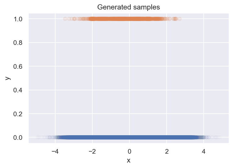
We are given a dataset of binary samples $y$ and a parameter $x$, and our task is to find out how the probability of $y=1$ changes with $x$, i.e., $p(y=1 \mid x)$ (we call this the event rate). We decide to plot your samples up in a scatter plot, and what we get is this:

1 million binary samples. With only 1000 positive samples, $y=1$ is a rare event.

Unfortunately, this tells us nothing about $p(y=1 \mid x)$. We can see that there are less positive samples for more extreme values of x, but there are also less negative samples. To see what’s going on, we make a histogram next:

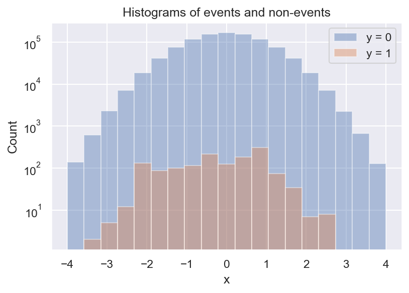
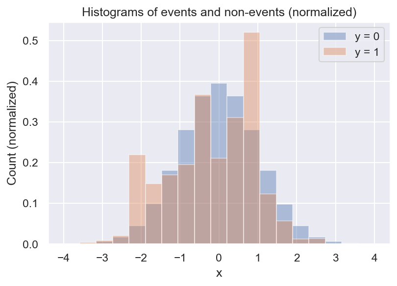
Histograms of positive and negative samples, raw counts (left) and normalized (right).

Now we see that there are always a lot more negative than positive samples, and we also see that there seem to be some local peaks in the distribution of $y=1$. But what we actually want is the frequency of $y=1$ relative to $y=0$. We can get a first estimate of $p(y=1 \mid x)$ by computing the ratio of the 2 histograms:

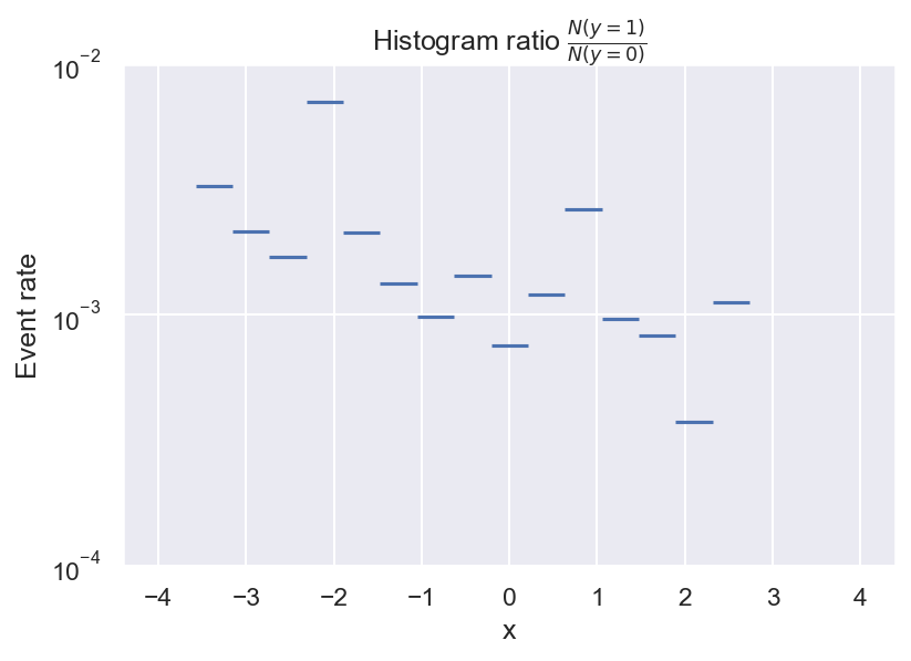
A first estimate of the event rate $p(y=1 \mid x)$.

This is pretty useful already: It looks like the event rate is higher towards negative values of x, and there seem to be 2 local peaks. But there are still some problems with this approach. For example, do we even have enough data to determine the event rate for every bin? What about bins with no positive samples? And how many bins should we choose?

Bayes to the rescue¶

Bayesian histograms address these issues by adding uncertainties to $p(y=1 \mid x)$. For this, we need to make some assumptions about the data generating processes.

We assume that, within each bin $i$, the number of positive samples $n^+_i$ is drawn independently with fixed probability $p_i$ (this is what we want to estimate) and number of negative samples $n^-_i$. Then, $n^+_i$ follows a binomial distribution:

$$ n^+_i \sim \operatorname{Binom}(n^-_i, p_i) $$

Our goal is to estimate $p_i$ via Bayesian inference. For this, we still need a prior for the variable $p$, which encodes our belief of what $p$ is before measuring any data (this also takes care of empty bins). A convenient choice is a beta distributed prior with 2 parameters $\alpha_0, \beta_0$:

$$ p(y=1) \sim \operatorname{Beta}(\alpha_0, \beta_0) $$

There are many ways to choose the prior parameters. Popular choices are complete ignorance ($\alpha_0 = \beta_0 = 0$; all values of $p$ are equally likely) and Jeffrey’s prior ($\alpha_0 = \beta_0 = 1/2$). In bayeshist, we use a weakly informative prior by default that ensures that the prediction of an empty bin is the global mean event rate with a big uncertainty.

Now we are ready to compute the posterior distribution of $p_i$. According to Bayes’ theorem, it is given by the normalized product of (beta) prior and (binomial) likelihood. A neat property of the beta prior is that it is conjugate to the binomial likelihood, so the posterior is a beta distribution, too:

$$ p(y=1 \mid n^+_i, n^-_i) \sim \operatorname{Beta}(n^+_i + \alpha_0, n^-_i + \beta_0) \tag{1} $$

To get uncertainties on our event rate estimates, all we need to do is to compute a credible interval of the posterior (1) via its quantiles. In Python this looks like this:

# compute number of positive and negative samples per bin
>>> n_plus = 10
>>> n_minus = 10_000_000

# Jeffrey's prior
>>> alpha_0 = beta_0 = 0.5

# define posterior
>>> p_posterior = scipy.stats.beta(n_plus + alpha_0, n_minus + beta_0)

# evaluate posterior mean
>>> p_posterior.mean()
1.0499988450012706e-06

# 98% credible interval
>>> p_posterior.ppf([1e-2, 1 - 1e-2])
array([4.44859565e-07, 1.94660572e-06])

This tells us that, with 98% certainty, the event rate for this sample lies between $4.5 \cdot 10^{-7}$ and $1.9 \cdot 10^{-6}$, with a mean value of $1.0 \cdot 10^{-6}$.

Computing quantiles of a beta distribution is very fast, so we can perform this calculation for every histogram bin with almost no additional compute cost. This is what bayeshist does to compute a Bayesian histogram.

from bayeshist import bayesian_histogram, plot_bayesian_histogram

bins, bin_posterior = bayesian_histogram(X, y, bins=20, pruning_method=None)
plot_bayesian_histogram(bins, bin_posterior)

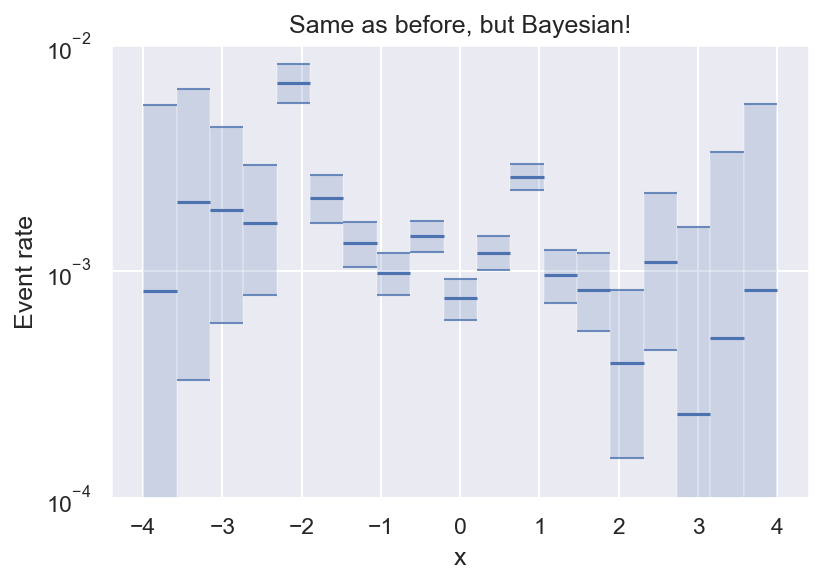
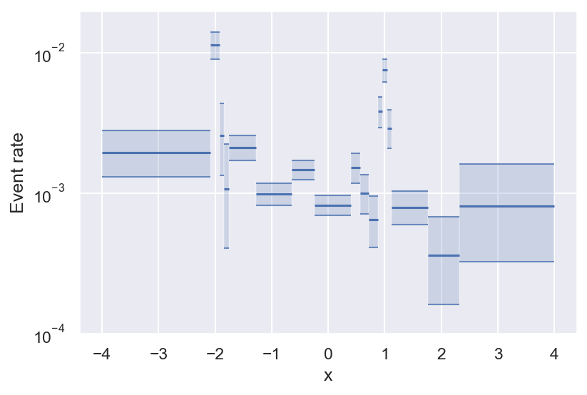
Bayesian histogram estimate of event rate $p(y=1 \mid x)$.

Now we have an estimate for all bins (even empty ones), and we can see that we have enough data to say that the variation we see for $|x| \leq 2$ is statistically significant.

But there is still one major open question: How many bins should we use?

If we use too many bins, the sample size per bin will be tiny, so our uncertainties will be huge.
If we use too few bins, there will be a considerable variation of $p(y=1 \mid x)$ within each bin, which means that one of our main assumptions (that the event rate is constant) is violated.

We address this in the next section.

Significant bins only!¶

If we can come up with a way to determine whether 2 bins are significantly different, we could start with a high number of bins and merge non-significant bins until we are left with an optimal binning. This is the main idea behind histogram pruning.

Imagine that we want to compare 2 bins with samples $(n_1^+, n_1^-)$ and $(n_2^+, n_2^-)$. We formulate the following hypotheses:

H1: Sample 1 is drawn from bin 1 with
$$ p_1 \sim \operatorname{Beta}(\alpha_1 = n_1^+ + \alpha_0, \beta_1 = n_1^- + \beta_0) $$
and sample 2 is drawn from bin 2 with
$$ p_2 \sim \operatorname{Beta}(\alpha_2 = n_2^+ + \alpha_0, \beta_2 = n_2^- + \beta_0) $$
H0: Both samples are drawn from the merged version of both bins with
$$ p_{tot} \sim \operatorname{Beta}(\alpha_{tot} = n_1^+ + n_2^+ + \alpha_0, \beta_{tot} = n_1^- + n_2^- + \beta_0) $$

Now we want to know: how much more likely is it to measure the samples under H1 compared to H0? To answer this, we have to compute the likelihood of each sample, while accounting for every possible value of the unknown event rate $p$ (the result is also called a Bayes factor). This is typically done by integrating out unknown parameters from the posterior (marginalization). In our case of a binomial likelihood with beta-distributed event rate, the result is a Beta-binomial distribution:

$$ n^+_i \sim \operatorname{Betabinom}(n^-_i, \alpha_i, \beta_i) $$

Now we can evaluate the likelihood of each sample under H1 and H0, and compute the ratio (Bayes factor). In Python code, this looks like this:

def sample_log_likelihood(n_plus, n_minus, alpha, beta):
    """Probability to measure `n_plus` positive and `n_minus` negative events"""
    sample_posterior = scipy.stats.betabinom(
        n_plus + n_minus, alpha, beta
    )
    return sample_posterior.logpmf(n_plus)

def sample_bayes_factor(n_plus_1, n_minus_1, n_plus_2, n_minus_2, alpha_0, beta_0):
    """Bayes factor to decide between separate and merged bins

    (higher values -> splitting more favorable)
    """
    alpha_1 = n_plus_1 + alpha_0
    beta_1 = n_minus_1 + beta_0

    alpha_2 = n_plus_2 + alpha_0
    beta_2 = n_minus_2 + beta_0

    alpha_tot = n_plus_1 + n_plus_2 + alpha_0
    beta_tot = n_minus_1 + n_minus_2 + beta_0

    return np.exp(
        sample_log_likelihood(n_plus_1, n_minus_1, alpha_1, beta_1)
        + sample_log_likelihood(n_plus_2, n_minus_2, alpha_2, beta_2)
        - sample_log_likelihood(n_plus_1, n_minus_1, alpha_tot, beta_tot)
        - sample_log_likelihood(n_plus_2, n_minus_2, alpha_tot, beta_tot)
    )

With this we can finally find the optimal number of bins! The algorithm works like this:

Start with a relatively high number of bins (for example 100).
Compare a neighboring pair of bins with samples $(n_1^+, n_1^-)$ and $(n_2^+, n_2^-)$. If the data is at least $\epsilon$ times more likely under H1, we do nothing. Otherwise, we revert the split by merging the 2 bins, and replace them by a single bin with $(n_1^+ + n_2^+, n_1^- + n_2^-)$.
Proceed with the next pair, or start over with the first pair when reaching the end of the domain.
Stop when no more neighbors can be merged.

This is how this looks in action:

Bayesian histogram pruning.

(If you prefer a Frequentist method, bayeshist also supports Fisher’s exact test to test whether the Beta distributions of neighboring bins differ significantly. The results are very similar.)

It works™¶

Before I show you an example of a case where Bayesian histograms work well, let me warn you loud and clear: You can only trust Bayesian histograms if their underlying assumptions are fulfilled. That is, events must occur independently, and $p(y=1)$ must be approximately constant within every bin. Histogram pruning can help with finding a partition that satisfies the latter condition, but comes with another caveat: the resulting bins are only reasonable if the parameter space is well resolved. If you have big gaps in your data coverage that miss a lot of variability of $p(y=1 \mid x)$, bins will be merged too aggressively. So in practice, it can be a good idea to use both pruned and unpruned Bayesian histograms.

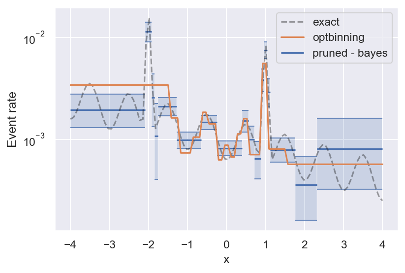
With that out of the way, here is the result on the example above, and the true event rate that the samples are generated from:

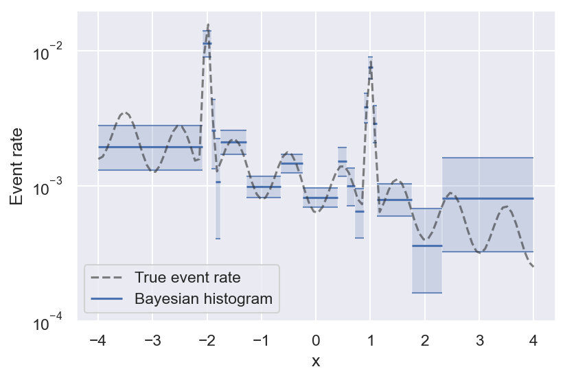
In this case, a pruned Bayesian histogram is a good representation of the true event rate.

See how bins get smaller the more variability there is in the true event rate? This is the effect of histogram pruning. If we had more samples, we could also resolve the oscillations towards the edges of the figure, but at this level of significance they are grouped into a single bin. Pruned Bayesian histograms are especially good at resolving local maxima in the event rate, which are often the most interesting regions — they even manage to get the full peak height right (within the uncertainty).

We can also compare pruned and unpruned histograms on this task:

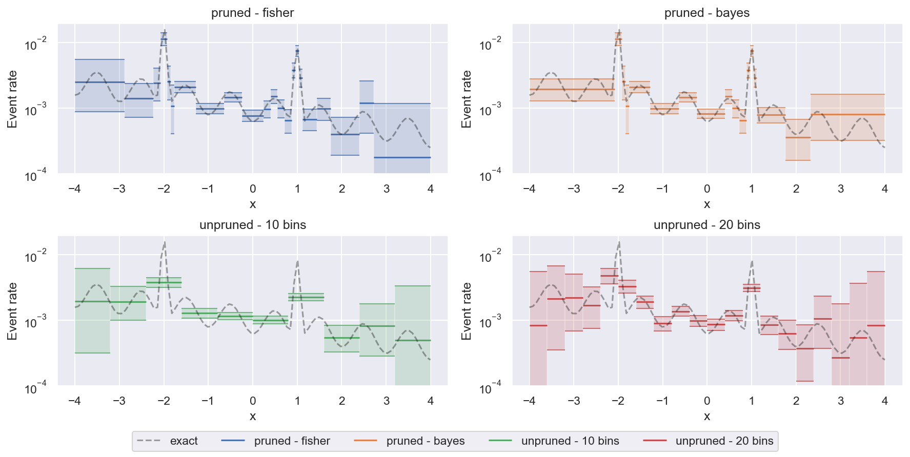
Output of pruned and unpruned Bayesian histograms on the same task.

Unpruned histograms are a bit more faithful when it comes to regions with very little data close to the edges of the figure (they show accurately where there are gaps in the data coverage with huge uncertainty). But pruned histograms are much better at resolving small-scale features with reasonable confidence.

Finally, we can compare the performance of bayeshist to the Python package optbinning. optbinning is much more powerful and does a lot more than estimating binary event rates. But on this particular task, it looks like Bayesian histograms work better:

Compared to optbinning, Bayesian histograms are able to resolve both local peaks at full height.

So why don’t you give bayeshist a try, and let me know what you think!